Catching up on Natural Language Processing with Deep Learning
Are you beginning in NLP, or just didn’t follow the latest advances? Wondering about OpenAI’s GPT2, the neural net that was too dangerous to be released? This article is for you. If you don’t know what NLP is or what machine learning is, you might have troubles understanding it. This is a technical article for machine learning students and practitioners.
Let’s start!
You can find the BibTeX references to most of the works cited in this text in this file.
- Introduction
- NLP tasks, datasets and evaluation
- Text preprocessing
- Language Models and RNNs
- Advanced architectures
- Universal language models and transfer learning
- Going forward
Introduction
Natural Language Processing is the field of machine learning that deals with language as humans speak or write it. It has of course roots in linguistics but it is now dominated by statistical models. With vision, it is one the fields at which humans are so good that we don’t realize the difficulty of the task. Consequently, like computer vision, it is now dominated by neural networks. Compared to classical machine learning models, they excel at tasks that we find intuitive, i.e. that are processed by our brain unconsciously. I will therefore focus specifically on NLP with deep learning.
A detailed tutorial on the matter already exists, but it’s quite long and a few years old now. A shorter and more recent one cannot hurt. You can also find a lot of information on Sebastian Ruder’s blog. I know about deep learning and have read enough about deep learning models for NLP to tell you about it, but I don’t have the knowledge to tell you about the linguistics side of things, which is necessary nowadays only for specific tasks such as part-of-speech tagging and constituency parsing.
This is a good time to get interested in NLP because 2018 has seen major breakthroughs. People finally obtained good performance in transfer learning, something that has been possible for years in computer vision (CV), with models trained on ImageNet. Recent powerful Universal Language Models can be trained unsupervised on large amounts of text data and then be reused with minimal fine-tuning for downstream tasks.
NLP tasks, datasets and evaluation
NLP has a large variety of tasks. Each of them represents a step towards machines understanding human language. Some of the main ones, along with the corresponding datasets and metrics, are listed below:
- language modelling: training a language model amounts to building a generative model for language (see Language Model for details). It is one of the most generic and popular NLP tasks. It is used for natural language generation. An unsupervised task, it allows to train a language model on corpora of text found on the internet. It makes language modelling one of the few tasks in AI for which virtually unlimited data is available. To train GPT2 (see this part), OpenAI used 40GB of text scraped on the internet1. The metric reported is the perplexity, which is the exponential of the entropy of the distribution defined by the model on the text. Intuitively, it represents how confused (perplexed) the model is in predicting the next word: a perplexity of \(k\) means the model is as uncertain as if it had to choose uniformly at random between \(k\) words. Lower is better;
- machine translation (MT): the acronyms SMT and NMT are often used to talk about Statistical MT and Neural MT. NMT consistently outperforms SMT nowadays, at the cost of poorer interpretability. Results in a given language pair are heavily influenced by data availability, but training MT models without parallel data is an active research area. International organisations such as the EU and the UN are excellent sources of high-quality translations. The metric used for assessing translation quality is BLEU (BiLingual Evaluation Understudy). It compares the model’s output to a number of reference human translation and quantifies how well \(n\)-grams overlap. Higher is better. The METEOR metric is sometimes preferred;
- sentiment analysis: classifying to what sentiment a piece of text corresponds. The popular IMDb dataset asks to classify whether movie reviews are positive or negative;
- question answering (QA): there are several tasks of QA. Most relevant to deep learning is extractive QA, meaning the answer to the question is a chunk of the contextual text given to the model. Other types include abstractive QA, where the model must generate the text of the answer, knowledge-base and logic-base QA. The most popular datasets are SQuAD and the more recent SQuAD 2.0. A leaderboard of the best-performing models is maintained. The metrics reported are the percentage of exact match between the model’s answer and one of the target answers, and the F1 score;
- named entity recognition (NER): the task of tagging entities in text with types. For instance, a NER system can be used to find people or places mentioned in a piece of text. F1 score is used.
- summarization: contracting a document into a shorter version while preserving meaning. To automatically assess summary quality, the ROUGE (Recall-Oriented Understudy for Gisting Evaluation) score is used. Several versions of ROUGE (ROUGE-\(n\), ROUGE-L, etc.) are available, each mesuring recall between subsequences of model prediction and reference summaries.
This list if far from exhaustive. A good resource to find datasets as well as SOTA results for a large number of NLP tasks is this one.
Text preprocessing
Classical preprocessing steps
In order to ease the task of computers, it is usual to clean the text as preprocessing. The first step is tokenisation, separating the text into tokens. A token is the basic unit of sense for the model, usually words but sometimes characters or subwords. Stop words are sometimes removed, depending on the application. Stop words are very frequent words that add little meaning to the sentence (e.g “the”, “and”, “of”). For basic sentiment analysis, one doesn’t need to know the precise grammatical structure of the sentence as long as informative words like “excellent” or “terrible” are kept. Of course this exposes us to missing more subtle formulations, especially if a word like “not” is removed. Depending on the application, you can also stem or lemmatise the word, i.e. replace the word by its root. This amounts to removing the conjugation of verbs, the declension of nouns, and in some cases replacing the word with a more common synonym (“automobile” becomes “car”). One can also correct spelling, if bad spelling can hurt model understanding.
Text preprocessing seems to be becoming somewhat outdated in NLP with deep learning. Tokenisation remains necessary—even humans cut text into basic pieces, but now that truly enormous amounts of text are being used to train ever larger models, the computation overhead of preprocessing (especially lemmatisation) becomes both problematic and unnecessary. Indeed, the impressive statistical power of recent deep learning models, fed with more text than a human could read in a lifetime, allows these models to learn the meaning of all different conjugations, declensions or misspellings that are common enough to be relevant.
Word embeddings
Computers deal with numbers, not with human words. We need to encode the latter into computer language. The naive way to do so is one-hot encoding, also known as the localist representation. Each word has a specific index and is represented as a very sparse vector of the size of the vocabulary, whose only nonzero element is a one at the word’s index. It is extremely high dimensional, and all word vectors are orthogonal to each other. Thus, it is impossible to define a notion of similarity. The words are treated as unrelated categories. This is obviously unsatisfying, so more sensible vector representations have been designed. Word2vec is a distributed vector representation, built on the distributional hypothesis2. There are many resources to explain Word2vec, but I’m going to suggest Jay Alamaar’s blog post because other posts of his blog will be useful later. The basic idea is to train a linear neural network to predict a word given its context (CBOW) or the context given a word (skip-gram). The context here contains the few words surrounding the word in question. It is actually equivalent to extracting the principal components of the co-occurrence matrix with a few additional tricks, which is called GLoVe. Using distributed word embeddings allowed to significantly improve the performances of most NLP models. It was an early kind of transfer learning, although a shallow one, as a single layer is reused (the embedding layer).
Language Models and RNNs
Language Model
A language model (LM) is a generative model for language. It can estimate the probability of a word appearing by itself, that of a word being the next word given the previous words, or even that of a sentence. It defines a probability distribution over the vocabulary \(V\). Smart keyboards use simple ones to give next words suggestions. Google uses a more sophisticated one for query suggestion and in its new Gmail feature. If you’re trying to predict the word at position \(t\) given the previous words, the model gives you \(P(w_t | w_0, w_1, ..., w_{t-1})\). If you want the probability of a sentence, the chain rule of probabilities allows you to write it as : \(P(w_{0:t}) = \prod_{l=0}^{t}P(w_{l+1}|w_{0:l})\). Before Recurrent Neural Networks (RNNs) really took off, the use was to assume that a word at position \(t\) only depended on the \(n\) words preceding it. This is called the Markov assumption. It allows one to write: \(P(w_t | w_{0:t-1}) = P(w_t | w_{t-n:t-1})\). For reasonable \(n\), e.g. 2 or 3 (5 is the maximum), one can simply count all the occurrences of the \(n\)-grams (tuples of \(n\) words), and estimate probabilities by normalizing by the total word count. If one wanted a fancier model, one could use a Hidden Markov Model (HMM), which exploited the Markov property with hidden variables. Although the Markov assumption is not entirely unreasonable — that’s what smart keyboard use and their pretty useful — we can easily see its limits when we want to deal with long term dependencies.
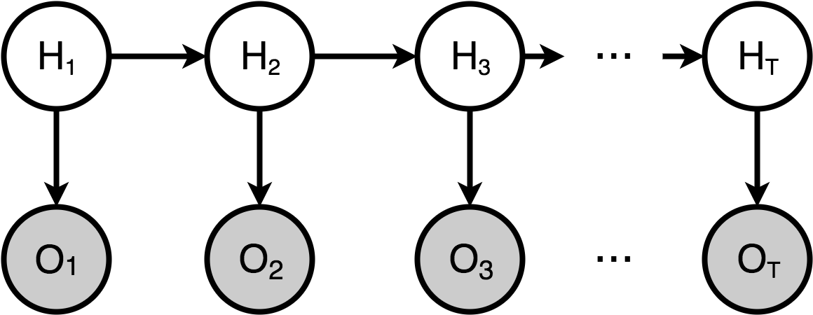 Example of Hidden Markov Model. Each hidden state only depends one the one preceding it. Although HMMs have been replaced by RNNs in NLP, there are very rich models that have many applications.
Recurrent neural networks and LSTMs
RNNs maintain an internal state that is updated at each new token. It is updated and not replaced, meaning it theoretically lifts the Markov assumption. However, due to gradient vanishing issues, vanilla RNNs are not great in practice. We use instead Long Short-Term Memory (LSTM) cells. Those are fancier RNNs designed to solve the gradient vanishing problem and have better long-term memory. They are a bit complicated, but you can read the great blog post by Chris Olah about them. More recent versions such as the Gated Recurrent Unit (GRU) have been proposed but LSTMs remained the default choice until transformers arose (see this section).
The training of an RNN for language modelling is as follows: at each time-step, the model is aware of the previous words and makes a prediction for the next one. This prediction comes from a softmax that outputs a discrete distribution over the entire vocabulary. Given the true next word, one can compute the cross-entropy loss, just as in normal classification. The losses for the different time-steps are then back-propagated through time (BPTT). Disappointingly, this term simply refers to the unrolling of the cell along the different time-steps (represented below). During BPTT, the weights matrix from the internal state to itself is multiplied by itself many times, as well as the gradient, which makes the training of vanilla RNNs unstable. LSTMs also solved this problem.
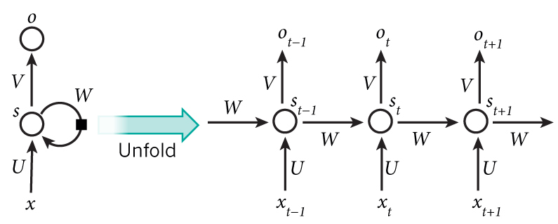 A vanilla RNN unfolded it time. Note the same weight matrices U, V and W used at each time-step.
Sub-word models
Although using entire words as tokens is most straightforward, especially in a language like English, this approach has shortcomings. How does one deal with out-of-vocabulary words or informal spelling? Humans can often get what a word means by looking at its spelling, even if it hasn’t been seen before. Using words as the smallest unit of sense in a LM doesn’t allow that. In Chinese, words are not space-separated; in German, words are composed to form nouns, the meaning of which is easily inferred from their constituent words; in languages with cases, a noun is declined according to grammatical rules, but keeps its meaning. To address these challenges, there has been research on using smaller units than words as tokens. There are three main strategies: working at the character level, using character \(n\)-grams (tuples of \(n\) characters), or using a hybrid model that models both words and sub-word units.
Character-level LMs work, and are the default way to go for ideogram-based languages such as Chinese. They also obtain very good results on morphologically-rich languages, such as German or Slavic languages. They are very slow, however, because the model processes about seven times more tokens and BPTT needs to be performed much further back in time than when tokens are words. Models based on character \(n\)-gram are a good compromise since morphemes3 are usually a few characters long. Nevertheless, pure sub-word models can be too biased towards syntax and spelling. For instance, they tend to translate proper names, which is sometimes desired but not always. Hybrid models have been developed to combine the power of sub-word models for unknown or rare words and that of word-level models for common words.
Advanced architectures
Seq2seq, Bi-LSTMS, stacked LSTMs
The straightforward way to use an LSTM is to pass it over a sentence and use the cell’s last internal state for further computation (e.g. a simple linear classifier). This architecture is known as an encoder because it encodes the sentence into a fixed-size vector. One can also form a decoder: from an initial vector state, the LSTM emits an output, which is re-fed as an input to the cell for the next step. The internal state of the LSTM is updated in the process. The decoder keeps emitting new tokens until it emits a specific stop signal. If the initial state is random, then one has a simple text generator, but otherwise the decoder forms a conditional language model able to generate text related to the information encoded in the initial state. We can combine an encoder and a decoder to get what is creatively called a sequence-to-sequence (seq2seq) or encoder-decoder architecture (same paper as GRU). The encoder maps the input from one domain to a common representation, and the decoder maps it from the common representation to another domain. This applies very naturally to machine translation (MT, illustrated below), but also to image captioning if the encoder is a computer vision model. An encoder-decoder model can be learned end-to-end, since the gradient can flow from the output of the decoder to the first layer of the encoder just as in a simpler neural network. This allows both parts to learn automatically the common representation.
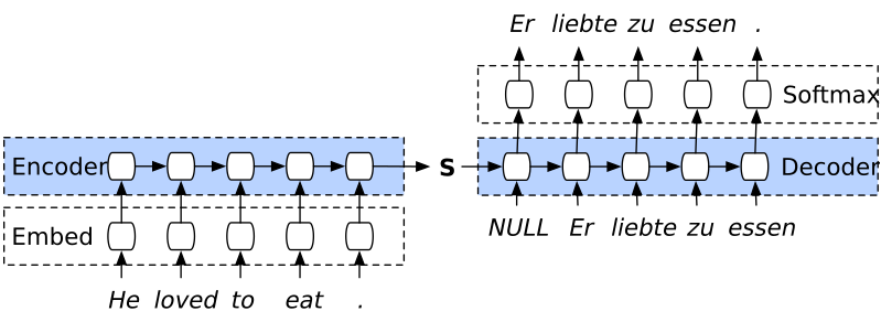 A sequence-to-sequence model for English-to-German translation. During training, the correct translation is provided as input to the decoder, no matter what words it actually outputs. At test time, the word emitted at position \(i\) is fed as input at position \(i+1\). A mechanism called beam search is used to ensure varied and coherent output.
LSTMs are not perfect, however; in particular, they don’t have such a good long-term memory. They can forget the beginning of the sentence by the time they get to the end. For MT, the simple trick of reversing the reading direction of the encoder improves performance; the start of the original sentence is then very close to that of its translation. This doesn’t solve the so-called bottleneck problem, however, which is that encoding sentences of varied lengths into fixed-size representations is hard. A solution is to use a bidirectional LSTM (Bi-LSTM). A Bi-LSTM is actually two LSTMs, one reading from left to right and the other from right to left. Their internal states are concatenated. The problem is that a Bi-LSTM doesn’t produce a fixed-size representation any more, which calls for additional design choices (e.g. a pooling function or an attention mechanism, see Attention and the Transformer). Finally, note that an LSTM, or even a Bi-LSTM, is still a shallow neural network when considered at each time-step: it comprises only one layer, or two counting the word embedding layer. This is in stark contrast to the CNNs with dozens of layers used in modern CV. To enable the abstract representations that depth permits, one can stack LSTMs on top of each other.
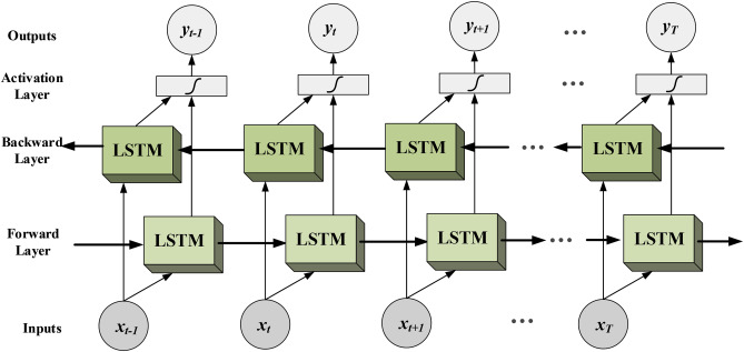 Bidirectional LSTM.
Convolutional neural networks for NLP
Another option to address the bottleneck problem is to look at a sliding window of a certain size, compute an encoding at each position, and pool over the positions to get a fixed-size encoding. This is similar to pooling the hidden states of an LSTM, except that one can look at several words at once, i.e. \(n\)-grams. The major advantage is that it is parallelisable, unlike an RNN. Computing something over a sliding window is in essence a 1D-convolution, so the network is now a CNN. Because CNNs are much faster than RNNs, we can also make them deeper—one rarely stacks more than three LSTMs. Good results have been obtained in this way, but it seems CNNs never established themselves as the way to go for NLP, probably because of transformers.
CNNs are also useful for sub-word models. They speed up computations and the concept of sliding window naturally lends itself to character \(n\)-grams.
Attention and the Transformer
Among the design choices available to map the internal states of a Bi-LSTM to a fixed-size representation, one can compute the mean or max element-wise, concatenate both, or use attention. Attention allows the model to attend more or less to words depending on a query. When you have a text in front of you and someone asks you a question about its content, you will pay attention to different words in the text, and just before answering, your attention will be maximally focused on the few words that you think give the answer. Attention in deep learning stems from that idea. In a neural network, an attention mechanism forms a weighted average of the internal states at different time-steps. The weights are the attention coefficients, and are computed using a softmax on attention scores. The latter are obtained, for instance, as the dot product of the corresponding internal state and a query vector. For question answering, this query vector may be an encoding of the question. For MT, it would be the internal state of the decoder at the current time-step. Attention scores can also be computed in other ways, e.g. with a learnable weight matrix in the middle of the two vectors.
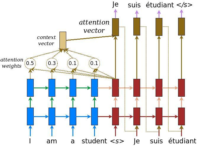 Attention mechanism for English-to-French translation. We see how much the model attends to each word in the English sentence when emitting a single token of the translation.
As we saw, the inherently sequential nature of LSTMs and Bi-LSTMs make them hard to parallelise, and storing all the states of a Bi-LSTSM raises memory issues. To solve this, Google researchers designed the Transformer. An excellent resource to understand this paper is Alexander Rush’s article. In addition, Jay Alamaar has again a nice blog post about it. The Transformer is essentially an encoder-decoder architecture, but it is purely based on attention mechanisms instead of recurrence and convolutions. It comprises six stacked encoder layers, each more complicated than a vanilla LSTM encoder. The output of the sixth encoder layer is fed to a decoder of the same depth. The encoder blocks are bidirectional, whereas the decoder blocks receive masked inputs in order to ensure that an output at position \(i\) only depends on known outputs at position less than \(i\). The architecture of a transformer is shown below. It is highly parallelisable, and yields much better performance than RNN-based architectures on a number of NLP tasks, especially when dealing with long-term dependencies. One of the main advances is multiheaded attention: instead of having one set of attention coefficients (one attention head), a transformer uses several. This allows it to deal with several queries at the same time: what is the subject of the sentence, what is the object, what verb are they linked to, and so forth. Transformers are now SOTA on most NLP tasks. They have also been used for image and music generation. Extensions of the Transformer have also been proposed, for instance in this work or this one. The latter resulted in OpenAI’s astounding MuseNet.
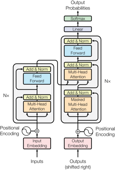 The original transformer architecture. Each encoder block contains a multi-headed attention layer followed by a linear layer, with residual connection and layer normalization. Each decoder layer first contains a masked multi-headed attention layer, masking words at position \(i\) and above in the target sequence if the model is predicting word \(i\), followed by a standard multi-headed attention and a linear layer. Each block is repeated \(N\) times, with \(N=6\) in the original paper. The positional encoding conveys the place of the word in the sentence.
Universal language models and transfer learning
ELMo and ULMFiT
Transfer learning (TL) is the concept of using the knowledge gained from training on a source task for solving a target task, for which less data is available, or for which we don’t want to train a model from scratch. Until recently, TL beyond word embeddings did not work well for NLP. Pretrained models were subject to catastrophic forgetting, meaning the model forgot all of its previous training during fine-tuning. This changed in 2018, with several papers achieving good TL performance. They are all based on so-called universal language models (ULMs). ULMs are simply language models trained on very large text corpora with no bias towards a specific task or theme, e.g. the whole of Wikipedia for one language (or several), or the BookCorpus, or both. The task of learning to predict the next word on such a large and varied body of text is very general (one might say universal), as much as, if not more than, ImageNet classification in CV. It is thus an excellent source task for TL.
Given this general task, we still need a way to actually transfer the knowledge gained in the ULM training to the target task. There are two directions to this: contextual word embeddings and the fine-tuning process itself.
The first was introduced by Embeddings from Language Models (ELMo). A similar idea has been proposed in the context of MT. It addresses the problem of polysemy: classical word embeddings cannot distinguish between the different meanings of the same word. The word “stick” will be represented by the same vector no matter what meaning of “stick” is being used. This vector will average the different meanings of “stick”, weighted by their frequency in the corpus used for training the word embeddings. This is a hurdle to language understanding by the model. To improve the latter, the word needs to be placed in context, i.e. associated with its neighbours. If you think of it, that’s actually what LSTMs and Bi-LSTMs do. Realizing this, the authors of ELMo trained two ULMs, a forward one and a backward one, using 3 stacked Bi-LSTMs. After training, the weights are frozen. When one wants to use ELMo for transfer learning, one then runs the frozen model over the target corpus, and gets three vectors for each word, one per LSTM layer. They are all contextual word embeddings, but capture different levels of abstraction—syntactic for the lower layer, semantic for the higher one. During TL, a weighted average of these vectors will be formed, with the weights learned from the target task. The resulting vector is the embedding of the corresponding word in context, and adapted to the target task. One can use ELMo as a drop-in replacement to vanilla word embeddings with any downstream model. This leads to significant performance gains on virtually all NLP tasks.
The second, Universal Language Model Fine-Tuning (ULMFiT), is a set of techniques that enabled reliable fine-tuning of ULMs. Contrary to ELMo, one can use ULMFiT to directly fine-tune the ULM itself to adapt to the target task instead of relying on a downstream model. It is not incompatible with ELMo but rather complementary. Still, it seems a more efficient kind of TL than pure contextual word embeddings, since the same model is used. This is illustrated by the great sample-efficiency of this technique: 100 datapoints are often sufficient to get good performance on the target task.
Using these techniques, one can train a big model once and then obtain quickly excellent performance on a number of tasks, just like ResNet models trained on ImageNet have been used for years in CV.
A battle of giants: BERT, GPT and GPT2, XLNet, and RoBERTa
The best-performing architectures for NLP nowadays are a mix of everything that works well: scaled-up transformers trained as ULMs on subwords, that can be fine-tuned using ULMFiT —or not— and provide contextual word embeddings, as well as sentence embeddings. Their names are GPT, BERT and GPT2. OpenAI’s GPT consists of 12 decoder blocks of a Transformer, without an encoder. Google’s BERT instead consists of 12 encoder blocks. Consequently, it has about the same number of parameters as GPT, but is bidirectional. The careful reader might wonder if a bidirectional LM doesn’t cheat by predicting words it has already seen. This is true, which is why the authors don’t train BERT on next token prediction. They instead mask 15% of the tokens and ask the model to guess those, solving the problem. If you’re wondering whether ELMo didn’t have this problem, it didn’t: the forward and backward LM in ELMo are independent, whereas BERT is a single bidirectional LM. As an additional objective, BERT has to tell whether a given candidate sentence follows the current one in the text, or is unrelated. This supposedly forces it to somewhat understand how sentences relate to each other, although this has been questioned, as we will see presently. BERT Large is a scaled-up version of BERT, with 24 encoder blocks. If you think BERT Large is huge, you’re right: 340M parameters. But OpenAI replied with GPT2: a direct scale-up of GPT with 48 decoder blocks and over 1.5B parameters. The model was so good at language generation that OpenAI didn’t release it, for fear of misuse. Once again, I link to Jay Alamaar’s blog for a good article. Obviously, these models take forever to train, especially if you don’t have TPUs. It is not that much of a problem, though, since we don’t need to train them from scratch, but only to use them for TL. Pre-trained versions are available on the web (except GPT2, but you can find smaller versions of it).
Since then, XLNet and RoBERTa came up. The first is BERT but with a fancier loss function, and it was SOTA for a time. It was then beaten by RoBERTa, which is also BERT, simply better trained. It doesn’t use the next sentence prediction task, questioning its usefulness.
The latest exciting advances that I am aware of aim at obtaining smaller models with the same performance as BERT. They use distillation; the original BERT is the teacher, and a lighter version of BERT is the student. The student is trained not on the targets from the dataset but on the probabilities predicted by the teacher, the soft targets. The student thus learns from the so-called dark knowledge that the teacher has accumulated during its own training. HuggingFace released DistillBert about a week before the publication of this post, and Google replied a few days later with the even smaller MiniBERT.
Going forward
NLP, and AI in general, advances blazingly fast. When I studied maths, we used to learn theorems that were over a century old. In one of my first machine learning courses, the teacher said: “that was proved last year.” Suddenly, I was in the research world. We were immersed in this constantly moving field, in which a result published one day might be contradicted or beaten a few days later; the example of DistillBERT and MiniBERT is just one among many. The richest firms on the planet were and still are investing billions in an arms race towards what the business world considers the most critical technological development of our century.
Solving NLP, building machines that can truly understand human language, will be a key step on the path to artificial general intelligence (AGI). Enabling reliable transfer learning in what has been called NLP’s ImageNet moment was certainly a major leap forward. Despite impressive results, BERT, GPT2 and the like are still far from truly understanding language. Said results come from their insane statistical power rather than an internal representation of the world. How could they know what words represent in our world? Would you ever learn Chinese by looking at ideograms, without ever seeing a translation? No, the best you could do would be to slowly learn that a specific ideogram often goes with another specific ideogram, or is often followed a few characters later by a third specific ideogram4. After days of careful study, you might be able to write something that looks like Chinese, but is gibberish. After months, you will be able to write a few coherent sentences, or even paragraphs. The longer you train, the longer the coherence length of your writing. But you still won’t have any idea of what you’re writing about. That’s exactly how ULMs work.
Further progress will require to associate words with real-life concepts, for instance to build models that not only see text but also images. This has been done for a while in image captioning and other subfields, but it needs to be scaled up the way language models were scaled up. I’m sure this is being done, and that the results will be both exciting and frightening. You might be wondering: “is that not still just associating some specific combination of pixels with a specific combination of token?” Yes it is, but hey, I guess that’s how we work.
For an open-source reproduction of this corpus: https://skylion007.github.io/OpenWebTextCorpus/. ↩︎
“You shall know a word by the company it keeps,” J.R. Firth ↩︎
In linguistic, a morpheme is the smallest unit of sense.} ↩︎
I don’t know anything about Chinese except that words can be one or two ideograms long and are not space-separated. ↩︎