Levelized Cost of Energy and Nuclear Power

25 Feb 2020

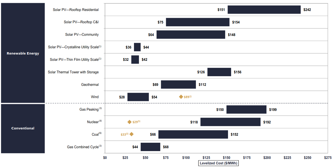
Investment firm Lazard has published the 13th version of their Levelized Cost of Energy (LCOE) assessment.

It has then been cited in an antinuclear report, and now I keep arguing over these numbers on Reddit with people who think we should ditch nuclear energy altogether because renewables appear so much cheaper in Lazard’s estimates. Yet, my country (France) has cheap, clean, and reliable electricity thanks to paid-for nuclear power plants. I’ve also seen this video (the whole channel is gold), that gives a good intuition of why nuclear power actually makes a lot of economic sense in the long run. To understand where this discrepancy comes from, I dug further into the subject.

How Lazard computes its estimates

Even though LCOE has evident flaws, such as not accounting for variability beyond the capacity factor, nor the end of life of the plant, I was still surprised by the large difference between the cheapest renewables and nuclear energy. I had a thorough look at the document, found a few assumptions that seemed off, and wanted to play with the model. I reproduced Lazard’s model in Python. You can find the code on my GitHub. I knew nothing about finance, so I learned just what I needed to know and asked a few questions to my M&A analyst friend Paul. Here is how LCOE works.

The methodology

Lazard’s methodology is described in this slide: 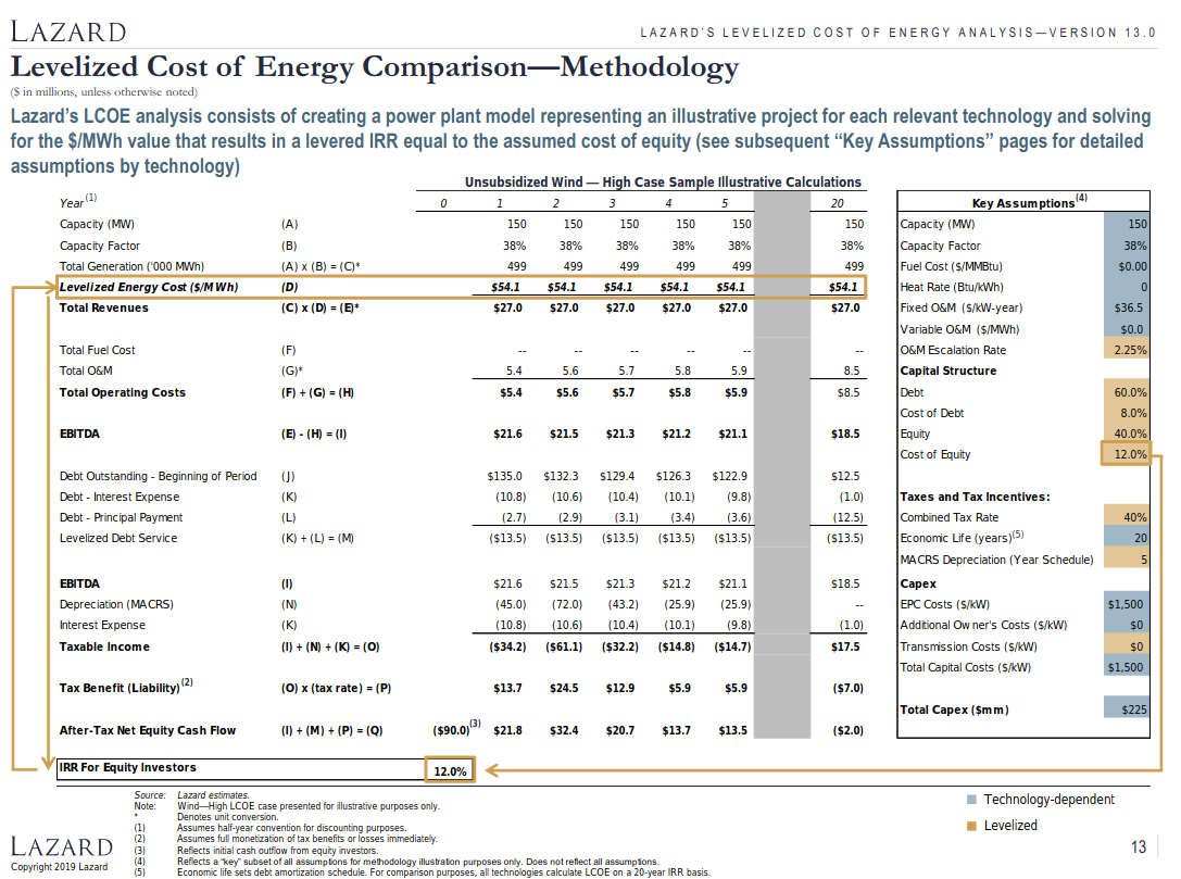Lazard builds a model of cash flows during the lifetime of the plant. On the right are assumptions that they have to make in order to estimate anything. The assumtions in blue are technology-dependent, while those in yellow are fixed for all technologies. At least that’s what it looks like, because I actually had to change the MACRS depreciation schedule to 20 for the conventional technologies (non-renewables), in order to match their results.

Some important numbers are those of the capital structure. The company that operates the plant finances it via borrowing 60% of the required capital at 8% interest from a bank, and the remaining 40% comes from investors who want back 12% each year on average. It’s a general rule: equity is always more expensive than debt. This debt structure defines the weighted average cost of capital, or WACC: \[WACC = P_{equity}C_{equity} + P_{debt}C_{debt}(1-t)\]

where \(P\) indicates the percentage, \(C\) the cost, and \(t\) the tax rate, because debt is tax-deductible. In this case, with a tax rate of 40%, the WACC is 0.4x0.12+0.6x0.08x(1-0.4) = 7.7%

Let’s now explain the model line by line. Just to be clear, in the slide above, monetary amounts are in millions, and negative amounts are in parenthesis.

• the first 3 lines including Year are part of the assumptions;
• Total Generation = Capacity x Capacity factor x 24 x 365 in MWh, /1000 in GWh;
• LCOE: what we’re looking for, we have to assume a value for now;
• Total Revenues (millions): Total Generation in MWh x LCOE / 1,000,000;
• Total Fuel Cost: 0 for renewables, for conventional you have to multiply the heat rate with the fuel cost and divide by a billion to get something in M$/MWh, and then multiply the result by Total Generation in MWh;
• Total O&M: Fixed O&M x Capacity + Variable O&M x Total Generation, divided by a million. That’s for year 1, and then you increase that by 2.25% every year;
• Total Operating Cost and EBITDA: the formulas they give are enough;
• Debt:
  1. multiply the capex by the percentage of debt (60%) to get year 1 of Debt Oustanding. Note that the capital cost already includes the construction time and accumulating debt over that period;
  2. compute the next two lines using functions called IPMT and PPMT, assuming the loan duration is the lifetime of the facility. As we will see, there’s something a bit fishy in these lines;
  3. Levelized Debt Service is the sum of the principal and interest payments;
  4. For the following years of Debt Outstanding, withdraw from year 1 the sum of the principal payments so far;
• Depreciation: it’s an accounting trick that allows a company to count the loss of value of its material capital (here the production means) as cash loss, which paves the way to tax deductions. We’ll see that it’s very important;
• Taxable Income has a formula;
• Tax Benefit: how much tax you pay. Note that it’s a liability, so you actually have to substract it in the calculation of the next line;
• After-Tax Net Equity Cash Flow: how much the investors earn each year. You can see in year 0 a number that corresponds to their initial investment, that is 40% of the capex.

Once you got all that filled up, you can compute the IRR of the investors. I’ll come back to what it is, but in practice it amount to calling the IRR function on the last line. The goal is then to adjust the value of the LCOE to find a IRR equal to the assumed equity cost of 12%. I do that by dichotomy, assuming the IRR is monotonously increasing with the LCOE. Sometimes it’s not the case, though, which I think is an artifact of the model rather than a real possibility. I avoided those cases.

Things I found suspicious

Even though I knew nothing about finance before this work, there are a number of things that make me believe that Lazard’s estimates might not be as solid or impartial as they seem:

• Why not make it clearer that the MACRS depreciation schedule is in the end technology-dependent? I don’t think they manipulated anything because, in my understanding, it’s set by law, but it clearly gives an advantage to renewables. Or perhaps it’s just obvious to professionals that renewables have the 5-year schedule and conventional the 20-year schedule;
• Their capacity factors for wind and solar are quite optimistic. They go from 21% to 34% for PV utily scale, and from 38% to 55% for onshore wind. Yet, looking at data from ourworldindata, the US Energy Information Administration, or the National Renewable Energy Laboratory, 15%-25% for solar and 25%-50% for onshore wind would have been much more honest;
• They use a facility life of 40 years for nuclear, whereas all reactors that are being built now are designed to operate at least 60 years. I suppose that’s because the nuclear project starts losing cash after 40 years according to the model (see the plot of the normalized cash flows later on), but perhaps it also means that the 2.25% escalation rate of O&M cost is not adapted to nuclear, or longer projects in general;
• Assuming the loan duration is the lifetime of the plant is wrong in many cases. I will explore that later;
• If you want to reproduce the exact same numbers as in the table above, you have to assume that the loan duration is the lifetime plus one year, and not the lifetime. If you do so, the loan is not completely paid for at the end of year 20. The numbers they show at year 20 are actually those of year 21. If you look at their version 12 estimates, you see that the last principal payment is not equal to the outstanding debt. When you make the calculations, it’s actually still the case in version 13, but they replaced year 20 with year 21;
• If you do what I just said to keep the exact same numbers, and compute the IRR of the last line, you find something like 8%, not 12% (and 54 $/MWh is the LCOE they report for that technology). I think that’s why my estimates are often a few dollars above theirs;
• From v12 to v13, they changed a few assumptions in a rather significant way without further justification (nothing is jutified actually). I specifically have in mind the 5-fold increase in variable O&M for nuclear. Not that I think the modification is necessarily wrong, but if after 12 iterations of that exercize, they still need to change numbers that much from a year to another (for a technology that’s not moving as fast as renewables I mean), it’s to me an indication that the initial work of finding the values to start with may not be rock solid;
• Finally, the IRR is computed on the first 20 year no matter the lifetime of the project. I suppose that’s because Lazard want to tell investors how well off they will be 20 years from now depending on their energy investments, but it doesn’t sound fair to long-living plants.

Despite these pointing to the possibility of the producer of this report having a slight bias towards renewables, I think we can rely on these estimates. I tried correcting for some of those things and it didn’t change much to the end result. I didn’t understand why at first, but then I realized it was because of the financial concepts I’m going to explain now.

Finance 101 and why investors are short-sighted

Let’s focus on the last row, the after-taxt net equity cash flow. It’s negative if investors inject money into the project, and positive if the project earns them money. The first element is always negative, and the following ones should most of the time be positive. Let’s call it \(C_t, t=0...n\), where \(n\) is the lifetime of the project, and \(t\) is the year number. \(C_0\) is the initial investment and is very negative. Then you might think that the value of the project, that we will call \(NV\) for Net Value, is the sum of the net cash flows: \[NV = \sum_{t=0}^nC_t\]

It is obvious that, as long as the project makes money, the longer its lifetime, the better. We can take an example: if our initial investment is 100 and we earn 10 every year, i.e. \(C_0\) = -100 and \(\forall t>0, C_t=10\), then \(NV=0\) after 10 years, 100 after 20 years, and 100 more per additional decade.

But that’s not how investors work. They have other potential investments, and if they can make more money on those, they have no reason to invest in this particular one. Let’s say they can make an annual return of \(r\) on other projects. Then our project needs to earn them a return of \(r\) or more to be of interest. This is captured by the Net Present Value: \[NPV = \sum_{t=0}^n\frac{C_t}{(1+r)^t}\]

The NPV is the sum of the cash flow discounted by the rate \(r\), that we call here is the discount rate. Investors have an interest in putting their bets on the project only if \(NPV>0\), otherwise they would have been better off putting them somewhere else. Our example project earns them 10% a year, so here \(NPV\) will be positive if \(r<0.1\) and negative if \(r>0.1\).

It totally makes sense for investors, but since \(r>0\), the future cash flows are discounted exponentially with their year number. It means profits made far into the future count a lot less, because investors expect to make a lot of money by then anyway. To visualize that, we can plot the NPV of our example as a function of \(n\) for a few different values of \(r\).

While a low discount rate allows to see the value of the investment far into the future, a higher one leads to no virtually no difference between the NPV of a project that will keep making money for 100 years and one that will stop after 20 years. The higher the investors’ annual return, the shorter-sighted they are. Once again, it’s perfectly rational for investors to reason like this, that’s not my point.

Before pursuing, I must complete my ultra basic intro to finance with the definition of the IRR. It is the discount rate such that: \[NPV(IRR) = \sum_{t=0}^n\frac{C_t}{(1+IRR)^t} = 0\]

To find the IRR, you multiply this equation by \((1+IRR)^n\), and you end up with a \(n\)-degree polynomial, of which you have to find the roots. There is no simple formula, so you have to use an optimization procedure, which can fail in some cases.

Lazard’s model assumes that the investors can make slightly less than 12% in other projects. They will invest in a given energy projects only if its NPV is positive, so that project must earn them an average annual return of 12%. So we must adjust the LCOE to find the series of cash flows that will have an IRR of 12%. You can see on the graph above why computing it on only 20 years and not on the whole facility lifetime doesn’t change much.

How depreciation makes renewables more attractive

As I said, depreciation is an accounting process in which an assets loses its value over a period of time. Importantly, it is counted as a cash loss for the company, which reduces its benefits, and therefore the taxes it has to pays, whereas there is actually no loss of cash. Thus, it can increase profit quite a lot. I personnally find it rather scandalous that taxpayers pay so that companies can replace their assets once in a while, whereas individuals just have to deal with them aging, but that’s not the topic.

There are several schedules for depreciation. The one used here is the Modified Accelerated Cost Recovery System (MACRS). Again, it’s not clear reading Lazard’s document, but renewables projects are depreciated over 6 years (which corresponds to the MACRS year schedule 5, don’t ask me why), and the others are depreciated over 21 years. For example, here are the percentages of the initial asset value lost each year in the 5 year option: 20%, 32%, 19.2%, 11.52%, 11.52%, 5.76%. They can seem absurdly arbitrary, but they actually come from an underlying process that makes sense.

You can’t see it on Lazard’s example because you don’t see the cash flow after year 5, but depreciation actually has an enormous effect on it. Here’s an excerpt of my model applied to the high wind onshore case, that of the methodology slide (keep in mind that I have slightly different numbers compared to Lazard for reasons I explained above).

Year	Depreciation	Tax_benefit	Net Equity Cash Flow
1	-45	13	23
2	-72	24	33
3	-43	12	21
4	-26	5.2	14
5	-26	5.2	14
6	-13	-0.1	8.8
7	0	-5.4	3.4

After year 7, the net equity cash flow keeps decreasing because of the escalating O&M costs, until it becomes slightly negative. In this example, the cash flow is divided by 5 after the asset is fully depreciated compared to the average of the depreciation period. But remember, to the investor, these first 6 years count a lot more than the following 14 in the life of the project. We can actually compute how much of the positive part of the NPV (without the inital investment) comes from them. We actually want two numbers: how much would come from them in our initial example of identical cash flow every year (assuming a lifetime of 20 years), and how much comes from them in the high wind case, taking into account depreciation.

Discount rate	Uniform case	High wind case
2%	34%	87%
5%	41%	89%
10%	51%	92%
12%	55%	93%
15%	60%	94%

At 12% equity cost, depreciation allows to gain almost 40 percentage points, making those first 6 years account for the quasi-totality of the NPV of the project (which is 0 by design, I’m talking about its “comeback from negative”).

If I change the MACRS year schedule to 20, cash flows are much more uniform over the lifetime of the project. My model gives a LCOE of 57.5 $/MWh with the original assumptions (54.1 $/MWh according to Lazard). The change in MACRS increases it to 71.7 $/MWh, and running a model with MACRS 20 and LCOE 57.5 $/MWh leads to a NPV of -31 M$.

As I said, I don’t think that’s Lazard trying to make renewables appear cheaper than alternatives, because in my understanding, the MACRS schedule is set by law. There’s still something wrong, though: the shorter lifespan of most renewables compared to other technologies should be a disadvantage, yet it allows them to benefit from a more advantageous law that boosts their attractivity to investors. Actually, even solar thermal, which has a 35-year lifetime, is depreciated over 6 years, whethear gas power plants are depreciated over their entire lifetime of 20 years. This looks a lot like a subsidy to me, but I guess that’s not considered as such because depreciation is so ubiquitous. Although I don’t like the short-termism it encourages, it’s understandable: it helps renewables be more attractive than fossil fuels, and we’re not gonna depreciate a nuclear power plant in 6 years anyway. This is to me a clear indication that a different financing system is needed for nuclear, and that comparing the LCOE of renewables and nuclear assuming the same capital structure is somewhat dubious.

Changing some assumptions

Now that I’ve explained how we calculate the LCOE, I’ll present the results I obtained by correcting for some of the assumptions I found weird.

Let’s start with the initial values. We will focus on the most promising renewables, wind (onshore only for simplification) and utility-scale PV solar (thin film to take the cheapest), and nuclear. Here is a summary of a few numbers (Lazard’s estimates are in parenthesis):

Technology	Lifetime (y)	Low LCOE ($/MWh)	High LCOE ($/MWh)
Wind onshore	20	29 (28)	58 (54)
PV Utility Scale	30	35 (32)	42 (42)
Nuclear	40	121 (120)	198 (192)

You see that my model reproduces Lazard’s pretty well, so now we can keep going with my model. Anyway, we don’t have a choice.

The first thing we want to do is to compute the IRR over the lifetime of the facility instead of just 20 years. We know it won’t change much for now, but we at least want the possibility to see far into the future. Only nuclear changes to 119 - 194 $/MWh.

More realistic capacity factors

As I said, I wasn’t so happy with their capacity factors, so I changed their range from 38%-55% to 25%-50% for wind, and from 23%-34% to 15%-25% for solar. Keep in mind that 50% for onshore wind is really exceptional, whereas 25% is the world average, so it’s not like I’m trying to make wind energy appear more expensive than it is. The new LCOE ranges are:

• wind: 32 - 87 $/MWh;
• solar: 48 - 64 $/MWh.

Just to give you an idea, here are the cash flows for the low case assuming the parameters above. I had to normalize them by dividing by the initial capital injection from equity because projects scales are different, especially nuclear.

We clearly see the effect of depreciation in all 3 projects, but it’s much starker in the renewable ones. As we already saw, most of the money made by the investors is made in the depreciation period. For information, with that cost of capital, depreciating renewables over 20 years yields these ranges of LCOE:

• wind: 40 - 109 $/MWh;
• solar: 62 - 84 $/MWh.

This graph also justifies the 20-year IRR calculation, since the profits from nuclear are less substantial after it’s depreciated, especially with a high discount rate. You can also see here why Lazard didn’t take a longer lifetime for nuclear.

Sensitivity to the cost of capital

If the investor were a country planning the future of its energy system, how would it reason? Well, money may grow 10% a year for investors (less for countries of course), but energy doesn’t. Actually, with the phase out of fossil fuels, that still represent over 80% of world primary energy production, we’re likely to have less energy in the future than we have now, at least in developed economies. Everyone is hoping that GDP can be decoupled from energy use, but no one is planning on the continued exponential increase of energy supply. It’s obvious to everyone that a physical value cannot grow exponentially forever. It follows that energy is likely to be more valuable in the future than it is now in rich countries. Moreover, with such a large part of dispatchable generation that must disappear, dispatchable sources will become even more valuable. Thus, I’d argue that it would make sense to apply very low, if not negative, discount rates for nuclear, and slightly higher ones for renewables.

But let’s keep things on the same ground for now. Below, you can see the sensitivity of these technologies to the cost of capital. You can find a similar plot in Lazard’s document, but it’s not very legible.

We see the extreme sensitivity of the cost of nuclear to the cost of equity. It remains more expensive than solar and wind, though. With a debt cost of 2% and an equity cost of 3% (which is possible if the investor is a state), for a WACC of 1.9%, the new LCOE ranges are:

• wind: 23 - 61$/MWh;
• solar: 29 - 38 $/MWh;
• nuclear: 67 - 99 $/MWh.

The change decreased a bit the LCOE of solar and wind while it virtually halved that of nuclear. It’s interesting to note that nuclear is now in the price range of solar and wind with the original capital cost and 20-year MACRS schedule (last subsection).

I haven’t change the capital structure, 60% debt and 40% equity, because it breaks the model. For some reason, the IRR becomes non-monotonous as a function of the LCOE, which makes the optimization fail.

Amortized plants

With ever-increasing O&M cost, an assumption that I don’t necessarily agree with but can’t change without much more work in analyzing actual 0&M costs over time, and a loan duration corresponding to the lifetime of the plant, a longer facility life is not necessarily an advantage. There is no moment when you will stop repaying your debt and turn into a cash machine, plus the longer the loan, the more interests you will pay overall. I modified my model to allow for a loan duration shorter than the facility life.

Let’s assume the loan duration of the nuclear project is 25 years. I know this number is reasonable because it’s used in the video I linked at the beginning of this article, but I don’t know what is a good number for solar and wind. I think the fairest way is to make it a bit longer than their depreciation period as well, let’s say 8 years. With the original capital structure and cost, here’s what the normalized net cash flow looks like for the low estimate.

Once the debt is repaid, the different projects generate a lot of cash. Some of them go through a few years of negative cash flows, though; I’m not sure investors would allow such a configuration. I guess it depends.

This experiment did not pan out as well as I expected, as it actually increases the LCOE of all three options:

• wind: 24 - 65 $/MWh;
• solar: 32 - 43 $/MWh;
• nuclear: 70 - 104 $/MWh.

Obviously, paying back your debt in a shorter amount of time means that you pay more every year during that time, which tends to reduce the attractivity of doing so. But I expected that, will a low enough discount rate, the significant and lasting gain in cash flow after the loan is reimbursed would easily make up for that and lead to a lower LCOE. But even increasing the lifetime of the nuclear plant to 60 years had very little effect on its LCOE: 68 - 99 $/MWh.

What it means for our energy choices

I’m gonna be honest: I was persuaded that the changes I made would bring the LCOE of nuclear in the same range as that of solar and wind. The difference is not as stark once we account for potential differences in financial structures, correct the capacity factors, and have in mind the arbitrariness of depreciation, but still the LCOE of nuclear remains signifiantly higher than that of those renewables.

I’m probably biased towards nuclear, but this position comes from a long reflection and extensive research that led me to believe that nuclear is technically an intrisically superior source of energy than renewables (I know, the term “source” is not exactly right). In my vision, its density, potential abundance, and reliability make it a much better candidate than renewables for being the main source of electricity and heat in the future (without exclusivity, of course). Countries currently using a lot of nuclear have great electrical grids. Meanwhile, scenarios based mostly or only on renewables rely on things that are not there or proven yet, on imports, or on unpalatable demand management.

Lazard’s numbers explain why there is ten times more investments in renewables than in nuclear (a few hundred billions a year versus a few dozen). But why then is electricity twice as cheap in France as in Germany? We’ve seen that nuclear can be much more affordable with the right capital structure (it is estimated than the Britich Hinkley Point C project could have been half the price if financed by the state ¹). It’s true, however, that it has become more expensive over time in the West, whereas renewables prices have decreased sharply. Here is probably part of the explanation: the French nuclear plants were built for a much cheaper price than most new nuclear projects, and German renewables were paid at a higher price than they would be today. But the other part is because of things that aren’t captured by LCOE, like intermittency, grid stability, variable electricity prices ². Why would we even consider gas peaking plants otherwise?

So, should we ditch nuclear? No, we should make it cheaper. Renewables were expensive and we’ve put a lot of energy and money into making them affordable, because we knew they were worth it. Well, we also know that the energy transition will be much easier if we don’t throw away a major source of clean and dispatchable electricity. Moreover, there’s still an enormous margin of improvements for nuclear. Imagine: some generation III+ reactors that are being built now were designed in the 90’s without CAD.

Pressure groups have certainly contributed to making the cost of nuclear artificially high by forcing never-ending authorization procedures and aburdly high safety standards, by spreading fear of an energy that was already the safest, including accidents. I won’t hesitate to accuse them of aggravating climate change in doing so. They are responsible for easily dozens of billions of tons of CO2 that were emitted by coal and gas plants over the last decades, that would have never existed had nuclear continued its development unimpeded. And now, the oil and gas industry is of course very happy with the turn of events, as a large part of electricity will continue to come from the gas plants required by grids full of renewables.

I’m not against renewables, but I’m defnitely against 100% renewables scenarios, as they are inferior in basically every way to those with nuclear and renewables. There is a reason why the IPCC considers nuclear an important option. Now is time to listen to the right people for once, and start working on making nuclear cheaper instead of more expensive. There are basically two techniques: do like the French have done in the past and the Chinese are doing now, or bet on small modular reactors (SMRs).

The first is more adapted to planned economies with public operators and low cost of capital. The idea is twofold: cram many reactors (4, 6, 8) in a single plant to save some overhead cost, and build the same reactor over and over again. Learning by doing is significant for nuclear. It has worked very well for the French in the 70’s-80’s, and more recently for renewables. Unfortunately, it works in reverse: forgetting by not doing. It also happened to France, which explains the debacle of the EPR in Flamanville. Avoiding that requires to keep a constant activity of retiring old reactors and building new ones, and not just building all your reactors super fast and then be content with operating them for decades before starting to build the next generation. It’s easier to do with SMRs.

The second solution fits better into liberal economies. SMRs are, well, small and modular reactors. Small means their capacity if less than 300 MWe. Modular means that they are made from parts that are manufactured in an industrial fashion. A SMR can thus be built and assembled in factory, then shipped to its final location. While large reactors are akin to public works, whose cost increases over time, industrialization tends to decrease cost over time, as was the case for renewables. We could imagine a few reactors getting ouf of a factory every day, just as some factories churn out several airliners per day (I have a hard time believing it, but it’s true). Why are SMRs better for liberal economies? Well, the upfront cost is much less, the risk as well, the construction time too, and hopefully it will decrease the capital cost per MW of nuclear over time. All of those should boost the attractivity of nuclear to investors. I actually think this is super promising even for more centralized economies. NuScale is a prominent American start-up in the field, but Russia, China, and recently France are also in the game.

Abandoning nuclear energy because renewables have a better LCOE is way too risky: we don’t even know yet if a whole energy system entirely based on renewables is possible, or compatible with an industrial civilization. For such an important problem, failure is unacceptable. We must hedge our bets and keep exploring all options, especially when they’re as promising as nuclear.

1. Report from the British National Audit Office ↩︎

2. You can read this critique of LCOE, or this paper, for instance. ↩︎